If you search for “Lending Club default prediction” you will find notebooks reporting AUC scores of 0.90 and higher, while the published range for leakage-aware setups is 0.69 to 0.73. This project lands at 0.72, and understanding that gap turned out to be the most valuable lesson of the whole exercise: it comes down to what information the model is allowed to see. These are the decisions behind it, dead ends included.

The trap hiding in 151 columns

The Lending Club dataset has 2.26M loans and 151 columns. Here is the problem: most of those columns describe what happened after the loan was granted. Total payments received. Amounts recovered after collections. The borrower’s updated FICO score, months or years into the loan. Hardship and debt settlement programs.

If you train a model with those columns, you are training with the answer. A loan with low total payments obviously defaulted, but on the day the lender has to decide, that number does not exist yet. This is called data leakage, and on this dataset it is everywhere. The models scoring 0.90+ are almost always reading the future.

So the first and most important modeling decision had nothing to do with algorithms. It was one question, applied to 151 columns: did the lender know this on approval day? Twenty-eight columns survived.

Let the data answer your design questions

Three moments where a quick measurement replaced a guess:

The credit-bureau block. About 60 columns of detailed credit history looked promising, but they had massive missing values. Grouping missingness by loan year showed the pattern: 100% missing until 2011, half missing in 2012, complete from 2013. The columns were added to the platform’s schema in 2013; the missing values were structural, not random. Two different columns shared the exact same missing rate (0.519816), which is the fingerprint of a block that appears together. I dropped the block and kept the FICO score, which exists for the whole period and summarizes it.

The censoring problem. A 36-month loan granted in 2017 cannot be “finished” by the end of 2018, unless the borrower paid everything early or stopped paying almost immediately. So recent cohorts only contribute extreme cases. Measuring the share of finished loans per year made it visible: 100% for 2011-2013, 38% for 2017, 11% for 2018. That bias cannot be fixed, but it can be measured and declared as a limitation.

The US state. Default rates range from about 14% (Oregon) to 24% (Arkansas) among large states, so geography carries real signal and I wanted it in. Including it properly is not trivial: to avoid leakage, any grouping or encoding of states by risk has to be learned from the training set only. That needed more time than this project had, so the variable stayed out and geography moved to the improvement list.

Missing values that carry information

My favorite finding: 5.8% of applicants did not declare their employment length. Their default rate is 27%, seven points above the average. The missing value itself is a signal (“did not declare” says something about the applicant), so instead of imputing it, it became its own category. Meanwhile, the declared values barely matter: from “less than 1 year” to “10+ years”, the default rate only moves from 21% to 19%.

The lesson: before filling missing values, always check what the missingness itself predicts.

Accuracy lies when classes are unbalanced

Only 20% of finished loans defaulted. A model that predicts “everyone pays” scores 0.80 accuracy while detecting zero defaults. My first logistic regression did almost exactly that: 0.802 accuracy, 8.5% of defaults detected.

The fix starts with the metric, not the model. A missed default costs the lender the loan amount (about $15K). A wrongly rejected good payer only costs the interest (about $2.5K). With a 7:1 cost ratio, the metric that matters is recall of the default class, how many real defaults you catch, controlled by precision so the model doesn’t just reject everyone. With balanced class weights, the same logistic regression went from catching 8.5% of defaults to 64%, trading accuracy (from 0.80 to 0.66) for a model that is actually useful. Expected loss on the test set: from $804M with no model to $453M with the winner.

Model comparison

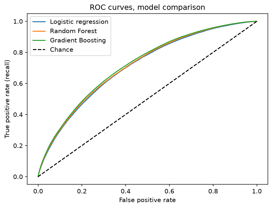
I compared logistic regression, a decision tree, a linear SVM, a random forest and gradient boosting, all with hyperparameter exploration and the same metric. The result surprised me: they all landed within a very narrow band (recall 0.63-0.68, F1 0.42-0.43).

Gradient boosting won on every metric (recall 0.678, AUC 0.720, trained in 24 seconds). But the honest reading of the table is that the ceiling is set by the information available at origination, not by the algorithm. When five very different models tie, stop tuning and look at your data.

Two side notes from the comparison:

• The random forest needed 4x the training time of gradient boosting to lose on every metric.
• The plain logistic regression delivered almost the same performance in 5 seconds, with coefficients you can explain. In a regulated environment like banking, that is a serious argument.

Room for improvement

Things this project left on the table: recalculating the debt-to-income ratio to include the new loan’s installment (a feature suggested in Namvar et al. 2018, the reference paper for leakage-aware work on this dataset); bringing geography in with state groupings learned on the training set; and tuning the decision threshold with a profit function in dollars instead of a fixed cutoff.

The full analysis, with all the numbers and figures, is in the repository.